
Introduction
This is a standard operating procedure for calibrating your AQY 1.
Contact Technical Support if you’d like Aeroqual to do the NO2 calibration calculation for you. The first calibration is free of charge for Aeroqual Plus customers.
To download the AQY 1 calibration template, click here.
-
-
The regulatory station should meet the following criteria:
-
It collects air quality data for all pollutants of interest (NO2, O3, PM2.5) and the data is available at 1 hour (or more frequent) average values.
-
The station has a secure and safe structure to mount the AQY 1 (e.g. roof railings).
-
There is mains power available for the AQY 1 at the station.
-
The pollutant concentrations (O3, NO2 and PM2.5) are expected to be reasonably high at the regulatory site for at least some of the days during the co-location. Ideally, there should be some hourly averaged values for O3 > 60 ppb, NO2 > 40 ppb and PM2.5 > 50 ug/m3.
-
If multiple stations are available, choose the one with environmental characteristics most similar to the project monitoring site of the AQY 1.
-
-
-
Install the AQY 1 on the regulatory station so the gas and PM inlets are as close as possible and at a similar height.
-
Connect the power.
-
If you're using Aeroqual Cloud, confirm the AQY 1 is connected and data is being logged.
-
If you're not using Aeroqual Cloud, connect via Aeroqual Connect and confirm data is logging correctly.
-
Confirm the date-time stamp of the AQY 1 matches the regulatory station.
-
If you're calibrating multiple AQY 1 units, consider using an external 3G Wi-Fi router to connect all AQY 1 monitors to Aeroqual Cloud and save on data costs.
-
-
-
Leave the AQY 1 to run for a minimum of 3 days to collect enough data for a valid comparison.
-
If pollutant data is low, you should extend the co-location interval.
-
If the regulatory PM2.5 hourly averaged data is noisy, you may need to use 24 hour-averaged data and will need to co-locate for a considerably longer time, perhaps 2 weeks.
-
If meteorological conditions are unusual during the co-location, such as the presence of fog, storms or wildfires, you should extend the co-location interval.
-
The longer you can leave the AQY 1 at the co-location site the better, as more data will be collected, improving the accuracy of the calibration.
-
-
-
Download the AQY 1 data and reference data and prepare the data for comparison by checking the following:
-
Ensure the date-time stamp for the reference station and the AQY 1 match. If not, make the required changes to align the AQY 1 data to the reference data.
-
Ensure the reference data and AQY 1 data are using the same units of measurement.
-
Check the reference data and remove any invalid data such as daily calibrations or maintenance.
-
Remove invalid data from the AQY 1 data, such as the warm-up period (first 4-6 hours of operation), any spikes or lost data from power issues.
-
You should have a pair of data sets which have the same number of data and are correctly synchronised.
-
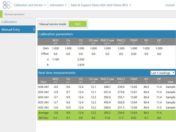
The AQY 1 uses the calibration parameters gain and offset which are applied to the readings to produce an accurate concentration. The form of the equation on the monitor is: [gas] = gain*(reading – offset).
-
-
-
Plot AQY 1 PM2.5 (y-axis) versus the regulatory PM2.5 (x-axis).
-
Calculate the slope and intercept from a linear least squares fit to the data.
-
Calculate the new AQY 1 gain and offset using the equations below:
-
New gain = old gain/slope
-
New offset = old offset + (intercept/old gain)
-
-
-
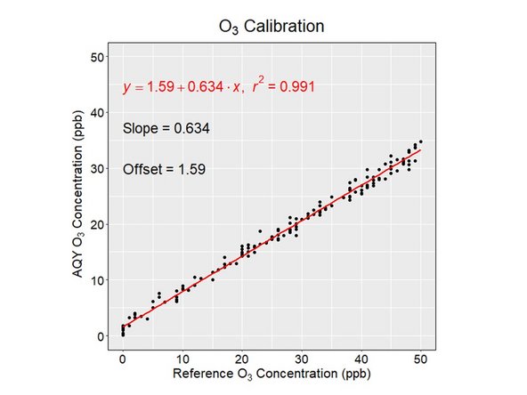
Plot AQY 1 O3 (y-axis) versus the regulatory O3 (x-axis).
-
Calculate the slope and intercept from a linear least squares fit to the data.
-
Calculate the new AQY 1 gain and offset using the equations below:
-
New gain = old gain/slope
-
New offset = old offset + (intercept/old gain)
-
The scatter-plot of ozone data shows a linear regression line with slope and intercept.
-
-
-
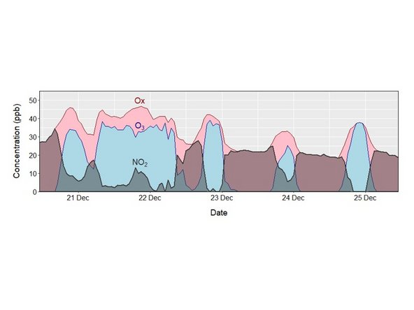
The AQY 1 NO2 measurement uses two sensors to calculate the NO2 concentration: a GSE Ox sensor and a GSS O3 sensor.
-
NO2 is calculated from the difference between the Ox and O3 sensors according to the equation [NO2] = [Ox] – 1.1* [O3].
-
The Ox and O3 sensor calibrations form part of the overall NO2 calibration and the sequence is important.
-
Since Ox sensor data isn't reported by the AQY 1, it must first be determined by back-calculation.
-
-
-
Back-calculate Ox using the equation: AQY 1 NO2 + (1.1*AQY 1 O3).
-
Calculate a new gain and offset for Ox using a linear least squares fit of AQY 1 Ox vs Ref (NO2 + O3).
-
Create calibrated Ox and O3 data (Oxcalibrated and O3calibrated) using the results of AQY 1 Ox vs Ref (NO2 + O3) and the O3 slope and intercept.
-
Calculate a NO2new dataset using the calibrated Ox and O3 data where NO2new = Oxcalibrated – 1.1*O3calibrated.
-
Undertake a linear least squares fit of NO2new to the reference NO2 to get slope and intercept for NO2.
-
Calculate the new NO2 gain and offset using the equations: New gain = old gain/slope and New offset = old offset + (intercept/old gain).
-
The time series plot shows NO2 is the difference between Ox and O3.
-
-
-
Upload new gains and offsets remotely via Aeroqual Cloud or onsite through Aeroqual Connect.
-
Once they're uploaded, validate the calibration by continuing to run the AQY 1 at the regulatory station and collecting 2-3 days of data.
-
Plot the scatterplots and confirm the slope and intercept of the linear regression line for each pollutant is close to 1 and 0, respectively. If they're significantly different, recheck your calculations.
-
If you can't see any errors, it’s possible the monitor has drifted and you may need to repeat the calibration process.
-
-
-
For extra help, watch our video.
-


For further support, contact Technical Support.
For further support, contact Technical Support.
Cancel: I did not complete this guide.
One other person completed this guide.

Team
